numpy.percentile

numpy.percentile(a, q, axis=None, out=None, overwrite_input=False, method='linear', keepdims=False, *, weights=None, interpolation=None)

计算指定轴上的数据的 q-th 百分位数.

返回数组元素的 q-th 百分位数.

参数:

a实数的类数组 (array_like)

可以转换为数组的输入数组或对象.

qfloat 的类数组

要计算的百分比或百分比序列.值必须在 0 到 100 之间(含).

轴{int, tuple of int, None}, optional

计算百分位数的轴或多个轴. 默认值是计算沿数组扁平化版本的百分位数.

outndarray,可选

用于放置结果的可选输出数组.它必须具有与预期输出相同的形状和缓冲区长度,但是如有必要,将强制转换(输出的)类型.

overwrite_inputbool,可选

如果为 True,则允许通过中间计算修改输入数组 a ,以节省内存. 在这种情况下,此函数完成后输入 a 的内容是未定义的.

methodstr, optional

此参数指定用于估计百分位数的方法. 有许多不同的方法,其中一些是 NumPy 独有的. 有关说明,请参见注释. 按 H&F 论文 [1] 中总结的 R 类型排序的选项为:

1. ‘inverted_cdf’

2. ‘averaged_inverted_cdf’

3. ‘closest_observation’

4. ‘interpolated_inverted_cdf’

5. ‘hazen’

6. ‘weibull’

7. ‘linear’ (default)

8. ‘median_unbiased’

9. ‘normal_unbiased’

前三种方法是不连续的. NumPy 进一步定义了以下默认"线性"(7.)选项的不连续变体:

• ‘lower’

• ‘higher’,

• ‘midpoint’

• ‘nearest’

在 1.22.0 版本发生变更: 此参数以前称为"interpolation",仅提供"linear"默认值和最后四个选项.

keepdimsbool,可选

如果设置为 True,则缩小的轴将保留在结果中,作为大小为 1 的维度. 使用此选项,结果将正确地广播到原始数组 a .

weights类数组,可选

与 a 中值关联的权重数组. a 中的每个值都根据其关联的权重对百分位数做出贡献.权重数组可以是 1-D(在这种情况下,其长度必须是 a 沿着给定轴的大小)或与 a 的形状相同.如果 weights=None ,则假定 a 中的所有数据都具有等于 1 的权重.只有 method=”inverted_cdf” 支持权重.有关更多详细信息,请参见注释.

在 2.0.0 版本加入.

interpolationstr, optional

method 关键字参数的已弃用名称.

自 1.22.0 版本弃用.

返回:

percentile标量或 ndarray

如果 q 是一个单独的百分位数且 axis=None ,则结果是一个标量.如果给出了多个百分位数,则结果的第一个轴对应于百分位数.其他轴是在 a 的归约之后保留的轴.如果输入包含整数或小于 float64 的浮点数,则输出数据类型为 float64 .否则,输出数据类型与输入的数据类型相同.如果指定了 out ,则返回该数组.

参见

mean

median

等效于 percentile(..., 50)

nanpercentile

quantile

等效于 percentile,除了 q 的范围在 [0, 1] 中.

注释

numpy.percentile 与百分比 q 的行为与参数为 q/100 的 numpy.quantile 的行为相同. 有关更多信息,请参见 numpy.quantile .

参考文献

[1]

R. J. Hyndman and Y. Fan, “Sample quantiles in statistical packages,” The American Statistician, 50(4), pp. 361-365, 1996

示例

Try it in your browser!

>>> import numpy as np
>>> a = np.array([[10, 7, 4], [3, 2, 1]])
>>> a
array([[10,  7,  4],
       [ 3,  2,  1]])
>>> np.percentile(a, 50)
3.5
>>> np.percentile(a, 50, axis=0)
array([6.5, 4.5, 2.5])
>>> np.percentile(a, 50, axis=1)
array([7.,  2.])
>>> np.percentile(a, 50, axis=1, keepdims=True)
array([[7.],
       [2.]])

>>> m = np.percentile(a, 50, axis=0)
>>> out = np.zeros_like(m)
>>> np.percentile(a, 50, axis=0, out=out)
array([6.5, 4.5, 2.5])
>>> m
array([6.5, 4.5, 2.5])

>>> b = a.copy()
>>> np.percentile(b, 50, axis=1, overwrite_input=True)
array([7.,  2.])
>>> assert not np.all(a == b)

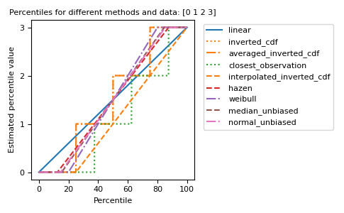
不同的方法可以用图形方式可视化:

import matplotlib.pyplot as plt

a = np.arange(4)
p = np.linspace(0, 100, 6001)
ax = plt.gca()
lines = [
    ('linear', '-', 'C0'),
    ('inverted_cdf', ':', 'C1'),
    # Almost the same as `inverted_cdf`:
    ('averaged_inverted_cdf', '-.', 'C1'),
    ('closest_observation', ':', 'C2'),
    ('interpolated_inverted_cdf', '--', 'C1'),
    ('hazen', '--', 'C3'),
    ('weibull', '-.', 'C4'),
    ('median_unbiased', '--', 'C5'),
    ('normal_unbiased', '-.', 'C6'),
    ]
for method, style, color in lines:
    ax.plot(
        p, np.percentile(a, p, method=method),
        label=method, linestyle=style, color=color)
ax.set(
    title='Percentiles for different methods and data: ' + str(a),
    xlabel='Percentile',
    ylabel='Estimated percentile value',
    yticks=a)
ax.legend(bbox_to_anchor=(1.03, 1))
plt.tight_layout()
plt.show()

Go BackOpen In Tab