numpy.random.RandomState.normal

method

random.RandomState.normal(loc=0.0, scale=1.0, size=None)

从正态(高斯)分布中抽取随机样本.

正态分布的概率密度函数,最初由 De Moivre 推导,200 年后由 Gauss 和 Laplace 独立推导 [2],通常被称为钟形曲线,因为它具有特征形状(参见下面的示例).

正态分布在自然界中经常出现.例如,它描述了受大量微小随机扰动影响的样本的常见分布,每个扰动都有其自己独特的分布 [2] .

备注

新代码应使用 normal 方法,该方法属于 Generator 实例;请参阅 快速入门 .

参数:

locfloat 或 floats 的类数组对象

分布的均值(“中心”).

scalefloat 或 floats 的类数组对象

分布的标准差(“宽度”或离散程度).必须是非负数.

sizeint 或 int 的元组,可选.

输出形状.如果给定的形状是例如 (m, n, k) ,则抽取 m * n * k 个样本.如果 size 为 None (默认),则如果 loc 和 scale 都是标量,则返回单个值.否则,抽取 np.broadcast(loc, scale).size 个样本.

返回:

outndarray 或标量

从参数化的正态分布中抽取的样本.

参见

scipy.stats.norm

概率密度函数,分布或累积密度函数等.

random.Generator.normal

新代码应该使用这个.

注释

高斯分布的概率密度为

\[p(x) = \frac{1}{\sqrt{ 2 \pi \sigma^2 }} e^{ - \frac{ (x - \mu)^2 } {2 \sigma^2} },\]

其中 \(\mu\) 是均值, \(\sigma\) 是标准差.标准差的平方 \(\sigma^2\) 称为方差.

该函数在均值处达到峰值,其“ spread ”随着标准差的增加而增加(该函数在 \(x + \sigma\) 和 \(x - \sigma\) [2] 处达到其最大值的 0.607 倍).这意味着正态分布更可能返回接近均值的样本,而不是远离均值的样本.

参考

[1]

Wikipedia, “Normal distribution”, https://en.wikipedia.org/wiki/Normal_distribution

[2] (1,2,3)

P. R. Peebles Jr., “Central Limit Theorem” in “Probability, Random Variables and Random Signal Principles”, 4th ed., 2001, pp. 51, 51, 125.

示例

Try it in your browser!

从分布中抽取样本:

>>> mu, sigma = 0, 0.1 # mean and standard deviation
>>> s = np.random.normal(mu, sigma, 1000)

验证均值和标准差:

>>> abs(mu - np.mean(s))
0.0  # may vary

>>> abs(sigma - np.std(s, ddof=1))
0.0  # may vary

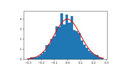
显示样本的直方图,以及概率密度函数:

>>> import matplotlib.pyplot as plt
>>> count, bins, ignored = plt.hist(s, 30, density=True)
>>> plt.plot(bins, 1/(sigma * np.sqrt(2 * np.pi)) *
...                np.exp( - (bins - mu)**2 / (2 * sigma**2) ),
...          linewidth=2, color='r')
>>> plt.show()

来自正态分布的 2x4 数组样本,均值为 3,标准差为 2.5:

>>> np.random.normal(3, 2.5, size=(2, 4))
array([[-4.49401501,  4.00950034, -1.81814867,  7.29718677],   # random
       [ 0.39924804,  4.68456316,  4.99394529,  4.84057254]])  # random

Go BackOpen In Tab