numpy.random.Generator.power

method

random.Generator.power(a, size=None)

从具有正指数 a - 1 的幂分布中抽取 [0, 1] 中的样本.

也称为幂函数分布.

参数:

afloat 或 floats 的类数组对象

分布的参数.必须是非负的.

sizeint 或 int 的元组,可选.

输出形状.如果给定的形状是例如 (m, n, k) ,则抽取 m * n * k 个样本.如果 size 为 None (默认值),则如果 a 是标量,则返回单个值.否则,抽取 np.array(a).size 个样本.

返回:

outndarray 或标量

从参数化的幂分布中抽取的样本.

提出:

ValueError

如果 a <= 0.

注释

概率密度函数为

\[P(x; a) = ax^{a-1}, 0 \le x \le 1, a>0.\]

幂函数分布只是帕累托分布的逆. 也可以看作是 Beta 分布的一个特例.

例如,它用于建模保险索赔的过度报告.

参考

[1]

Christian Kleiber, Samuel Kotz, “Statistical size distributions in economics and actuarial sciences”, Wiley, 2003.

[2]

Heckert, N. A. and Filliben, James J. “NIST Handbook 148: Dataplot Reference Manual, Volume 2: Let Subcommands and Library Functions”, National Institute of Standards and Technology Handbook Series, June 2003. https://www.itl.nist.gov/div898/software/dataplot/refman2/auxillar/powpdf.pdf

示例

Try it in your browser!

从分布中抽取样本:

>>> rng = np.random.default_rng()
>>> a = 5. # shape
>>> samples = 1000
>>> s = rng.power(a, samples)

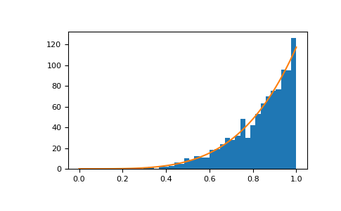
显示样本的直方图,以及概率密度函数:

>>> import matplotlib.pyplot as plt
>>> count, bins, _ = plt.hist(s, bins=30)
>>> x = np.linspace(0, 1, 100)
>>> y = a*x**(a-1.)
>>> normed_y = samples*np.diff(bins)[0]*y
>>> plt.plot(x, normed_y)
>>> plt.show()

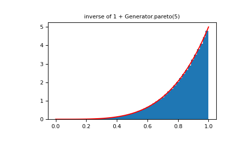
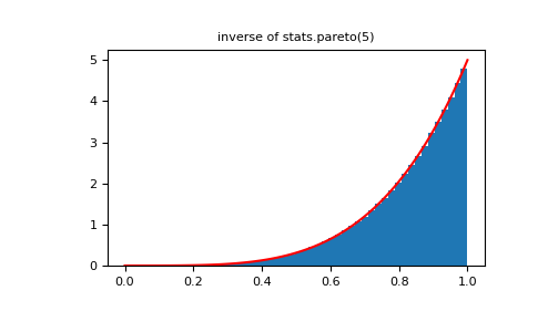
将幂函数分布与帕累托分布的逆进行比较.

>>> from scipy import stats  
>>> rvs = rng.power(5, 1000000)
>>> rvsp = rng.pareto(5, 1000000)
>>> xx = np.linspace(0,1,100)
>>> powpdf = stats.powerlaw.pdf(xx,5)  

>>> plt.figure()
>>> plt.hist(rvs, bins=50, density=True)
>>> plt.plot(xx,powpdf,'r-')  
>>> plt.title('power(5)')

>>> plt.figure()
>>> plt.hist(1./(1.+rvsp), bins=50, density=True)
>>> plt.plot(xx,powpdf,'r-')  
>>> plt.title('inverse of 1 + Generator.pareto(5)')

>>> plt.figure()
>>> plt.hist(1./(1.+rvsp), bins=50, density=True)
>>> plt.plot(xx,powpdf,'r-')  
>>> plt.title('inverse of stats.pareto(5)')

Go BackOpen In Tab